Soubor:3 phase rectification 2.svg

Velikost tohoto PNG náhledu tohoto SVG souboru: 397 × 600 pixelů. Jiná rozlišení: 159 × 240 pixelů | 317 × 480 pixelů | 508 × 768 pixelů | 677 × 1 024 pixelů | 1 355 × 2 048 pixelů | 624 × 943 pixelů.
Původní soubor (soubor SVG, nominální rozměr: 624 × 943 pixelů, velikost souboru: 120 KB)
| Tento soubor pochází z Wikimedia Commons. Níže jsou zobrazeny informace, které obsahuje jeho tamější stránka s popisem souboru. |
Popis
| Popis |
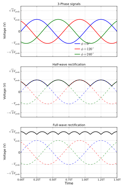
English: Waveforms for a typical 3-phase half-wave and full-wave rectifiers. The top plot shows the individual three phase signals, the middle plot shows the half-wave rectifier output in solid curve and the bottom plot shows the full-wave rectifier output in solid curve. The 'T' in time is the time period of individual signals and is the amplitude of each of the three input signals.
The diagram was created using python, matplotlib and numpy.
Русский: Формы сигналов трёхфазного одно- и двухполупериодного выпрямителей. Сверху - отдельные трехфазные сигналы, средний график - выход однополупериодного выпрямителя сплошной линией, нижний график - выходной сигнал двухполупериодного выпрямителя сплошной линией. T - период, U - напряжения. |
||
| Datum | |||
| Zdroj | Vlastní dílo | ||
| Autor | Krishnavedala | ||
| Další verze |
3 phase rectification 2.png
[]
.png:
.jpg:
|
||
| SVG vývoj | Tento vektorový obrázek byl vytvořen programem Matplotlib | ||
| Zdrojový kód | Python code
|


Licence
Já, držitel autorských práv k tomuto dílu, ho tímto zveřejňuji za podmínek následujících licencí:
Tento soubor podléhá licenci Creative Commons Uveďte autora-Zachovejte licenci 3.0 Unported
- Dílo smíte:
- šířit – kopírovat, distribuovat a sdělovat veřejnosti
- upravovat – pozměňovat, doplňovat, využívat celé nebo částečně v jiných dílech
- Za těchto podmínek:
- uveďte autora – Máte povinnost uvést autorství, poskytnout odkaz na licenci a uvést, pokud jste provedli změny. Toho můžete docílit jakýmkoli rozumným způsobem, avšak ne způsobem naznačujícím, že by poskytovatel licence schvaloval nebo podporoval vás nebo vaše užití díla.
- zachovejte licenci – Pokud tento materiál jakkoliv upravíte, přepracujete nebo použijete ve svém díle, musíte své příspěvky šířit pod stejnou nebo slučitelnou licencí jako originál.

|
Tento dokument smí být kopírován, šířen nebo upravován podle podmínek Svobodné licence GNU pro dokumenty verze 1.2 nebo libovolné vyšší verze publikované nadací Free Software Foundation. Dokument nemá neměnné části ani texty na předním či zadním přebalu. Kopie textu licence je k dispozici v oddíle nazvaném GNU Free Documentation License. |
Můžete si zvolit libovolnou z těchto licencí.
Historie souboru
Kliknutím na datum a čas se zobrazí tehdejší verze souboru.
| Datum a čas | Náhled | Rozměry | Uživatel | Komentář | |
|---|---|---|---|---|---|
| současná | 23. 9. 2011, 17:52 | | 624 × 943 (120 KB) | Krishnavedala | individual plots are now consistent with each other |
| 22. 9. 2011, 19:24 |  | 624 × 943 (114 KB) | Krishnavedala | final correction, hopefully!! | |
| 22. 9. 2011, 19:20 |  | 640 × 943 (116 KB) | Krishnavedala | corrected Time coordinates | |
| 22. 9. 2011, 19:04 |  | 623 × 943 (115 KB) | Krishnavedala | Corrected the waveforms for the full wave rectification. | |
| 1. 7. 2011, 00:06 |  | 599 × 944 (175 KB) | Spinningspark | Fixed correct use of italics. Fixed annotation outside boundary of image. Output waveform on top of input waveforms. | |
| 30. 6. 2011, 21:29 |  | 599 × 944 (111 KB) | Krishnavedala | removed "(sec)" from the x-axis label | |
| 30. 6. 2011, 21:27 |  | 599 × 946 (111 KB) | Krishnavedala | edits from suggestions in here | |
| 17. 6. 2011, 21:51 |  | 524 × 874 (142 KB) | Krishnavedala | thinner dashed lines | |
| 17. 6. 2011, 21:48 |  | 524 × 874 (142 KB) | Krishnavedala | all plots on the same scale to avoid confusion | |
| 8. 6. 2011, 19:18 |  | 594 × 946 (223 KB) | Krishnavedala | correction in the labels |
Využití souboru
Tento soubor používá následující stránka:
Globální využití souboru
Tento soubor využívají následující wiki:
- Využití na ca.wikipedia.org
- Využití na el.wikipedia.org
- Využití na en.wikipedia.org
- Využití na eo.wikipedia.org
- Využití na eu.wikipedia.org
- Využití na ja.wikipedia.org
- Využití na th.wikipedia.org
- Využití na zh.wikipedia.org