Soubor:Newton iteration.png

Původní soubor(2 406 × 1 978 pixelů, velikost souboru: 55 KB, MIME typ: image/png)

Popis

K tomuto obrázku existuje vektorová verze (v SVG). Pokud je lepší, používejte raději tu.

File:Newton iteration.png → File:Newton iteration.svg

Podrobnější informace o vektorové grafice najdete na stránce Commons:Transition to SVG.
Také si můžete přečíst informace o podpoře formátu SVG v MediaWiki.
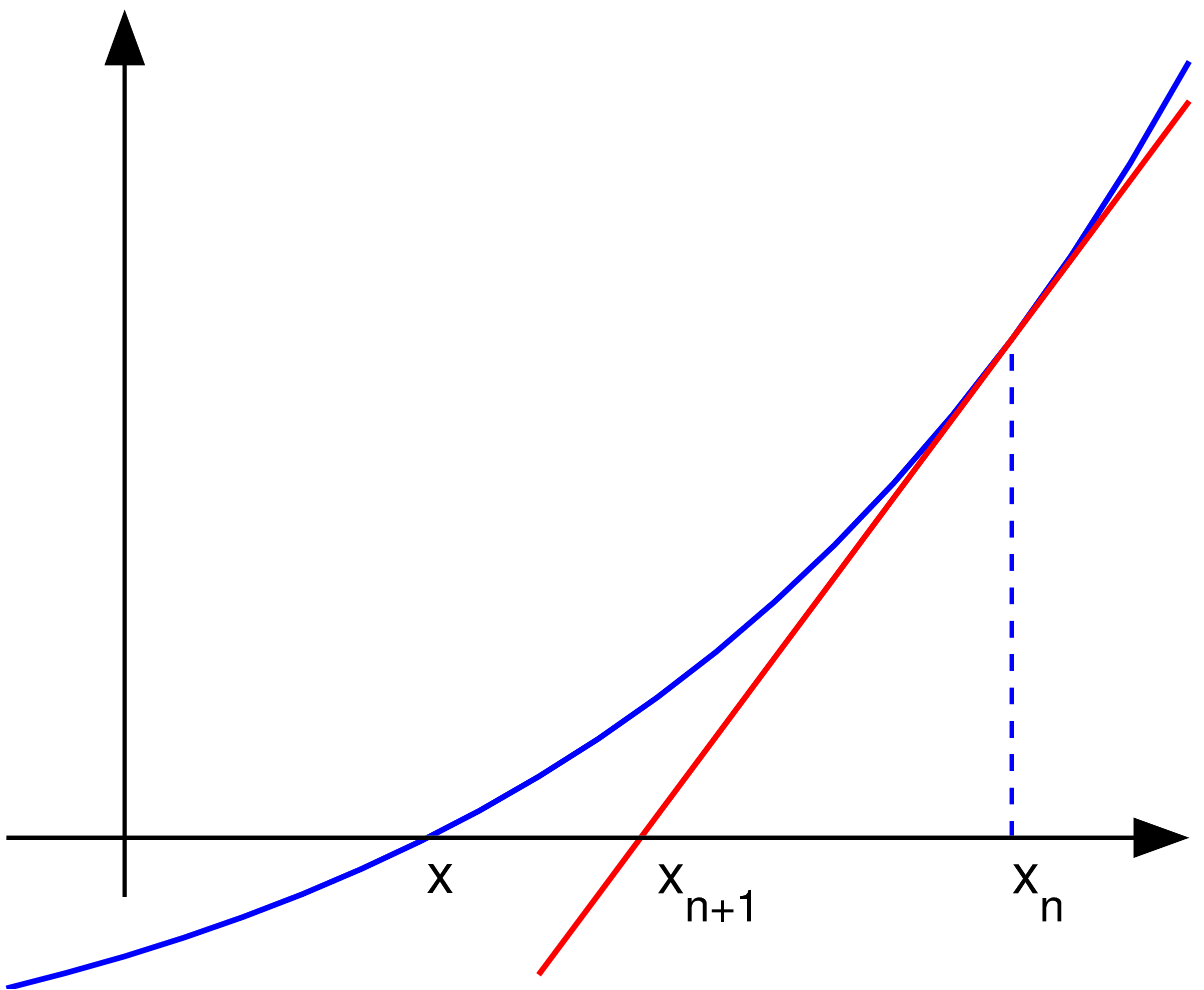
V jiných jazycích
Alemannisch  Bahasa Indonesia  Bahasa Melayu  British English  català  čeština  dansk  Deutsch  eesti  English  español  Esperanto  euskara  français  Frysk  galego  hrvatski  Ido  italiano  lietuvių  magyar  Nederlands  norsk bokmål  norsk nynorsk  occitan  Plattdüütsch  polski  português  português do Brasil  română  Scots  sicilianu  slovenčina  slovenščina  suomi  svenska  Tiếng Việt  Türkçe  vèneto  Ελληνικά  беларуская (тарашкевіца)  български  македонски  нохчийн  русский  српски / srpski  татарча/tatarça  українська  ქართული  հայերեն  বাংলা  தமிழ்  മലയാളം  ไทย  한국어  日本語  简体中文  繁體中文  עברית  العربية  فارسی  +/−
Nový obrázek ve formátu SVG

Popis Uploader graphed this with en:MATLAB (Illustration of en:Newton's method)
Datum 22. listopadu 2004 (first version); 2004-11-23 (last version)
Zdroj Na Commons přeneseno z en.wikipedia.
Autor Olegalexandrov na projektu Wikipedie v jazyce angličtina
PNG vývoj
InfoField
 
Tento PNG grafika byl vytvořen programem MATLAB
Zdrojový kód
InfoField

MATLAB code

(Newton iteration)
% illustration of Newton's method for finding a zero of a function

function main ()
   
a=-1; b=1;   % interval endpoints
fs=20;       % text font size

% arrows settings
thickness1=2; thickness2=1.5; arrowsize=0.1; arrow_type=1;
angle=20; % in degrees

h=0.1;  % grid size
X=a:h:b; % points on the x axis
f=inline('exp(x)/1.5-0.5');   % function to plot
g=inline('exp(x)/1.5');       % derivative of f
x0=0.7; y0=f(x0);             % point at which to draw the tangent line 
m=g(x0);
Y=f(X);                       % points on the function to plot
XT=-0.1:h:b; YT=y0+(XT-x0)*m; % tangent line

% prepare the screen
clf; hold on; axis equal; axis off

% plot the graph and the tangent lines
plot(X, Y, 'linewidth', thickness1)
plot(XT, YT, 'r', 'linewidth', thickness1)
plot([x0 x0], [0, y0], '--', 'linewidth', thickness2)

% axes
small=0.2;
arrow([a 0], [b, 0], thickness2, arrowsize, angle, arrow_type, [0, 0, 0])
arrow([a+small, -0.1], [a+small, 1.4], thickness2, arrowsize, angle, arrow_type, [0, 0, 0])

% text
H=text(-0.29, -0.06,  'x'); set(H, 'fontsize', fs)
H=text(0.1, -0.1,  'x_{n+1}'); set(H, 'fontsize', fs)
H=text(0.7, -0.1,  'x_{n}'); set(H, 'fontsize', fs)

% save to disk
saveas(gcf, 'newton_iteration.eps', 'psc2')

function arrow(start, stop, thickness, arrow_size, sharpness, arrow_type, color)

% Function arguments:
% start, stop:  start and end coordinates of arrow, vectors of size 2
% thickness:    thickness of arrow stick
% arrow_size:   the size of the two sides of the angle in this picture ->
% sharpness:    angle between the arrow stick and arrow side, in degrees
% arrow_type:   1 for filled arrow, otherwise the arrow will be just two segments
% color:        arrow color, a vector of length three with values in [0, 1]

% convert to complex numbers
   i=sqrt(-1);
   start=start(1)+i*start(2); stop=stop(1)+i*stop(2);
   rotate_angle=exp(i*pi*sharpness/180);

% points making up the arrow tip (besides the "stop" point)
   point1 = stop - (arrow_size*rotate_angle)*(stop-start)/abs(stop-start);
   point2 = stop - (arrow_size/rotate_angle)*(stop-start)/abs(stop-start);

   if arrow_type==1 % filled arrow

      % plot the stick, but not till the end, looks bad
      t=0.5*arrow_size*cos(pi*sharpness/180)/abs(stop-start); stop1=t*start+(1-t)*stop;
      plot(real([start, stop1]), imag([start, stop1]), 'LineWidth', thickness, 'Color', color);

      % fill the arrow
      H=fill(real([stop, point1, point2]), imag([stop, point1, point2]), color);
      set(H, 'EdgeColor', 'none')

   else % two-segment arrow
      plot(real([start, stop]), imag([start, stop]),   'LineWidth', thickness, 'Color', color);
      plot(real([stop, point1]), imag([stop, point1]), 'LineWidth', thickness, 'Color', color);
      plot(real([stop, point2]), imag([stop, point2]), 'LineWidth', thickness, 'Color', color);
   end

Licence

Public domain Olegalexandrov na projektu Wikipedie v jazyce angličtina, autor tohoto díla, jej uvolnil jako volné dílo, a to celosvětově.
V některých zemích to není podle zákona možné; v takovém případě:
Olegalexandrov poskytuje komukoli právo užívat toto dílo za libovolným účelem, a to bezpodmínečně s výjimkou podmínek vyžadovaných zákonem.


Původní historie souboru

Původní stránka s popisem souboru byla zde. Všechna následující uživatelská jména odkazují na projekt en.wikipedia.
  • 2004-11-23 19:55 Olegalexandrov 405×340×8 (14290 bytes) Scaled down the picture of Newton's method
  • 2004-11-22 21:34 Olegalexandrov 509×406×8 (16510 bytes) I graphed this with Matlab (Illustration of Newton's method) {{PD}}

Popisky

Přidejte jednořádkové vysvětlení, co tento soubor představuje

Položky vyobrazené v tomto souboru

zobrazuje

Historie souboru

Kliknutím na datum a čas se zobrazí tehdejší verze souboru.

Datum a časNáhledRozměryUživatelKomentář
současná25. 5. 2007, 05:23Náhled verze z 25. 5. 2007, 05:232 406 × 1 978 (55 KB)Oleg Alexandrov{{Information |Description=Uploader graphed this with en:MATLAB (Illustration of en:Newton's method) ==Source code== <pre> <nowiki> % illustration of Newton's method for finding a zero of a function function main () a=-1; b=1; % interva
13. 6. 2005, 01:11Náhled verze z 13. 6. 2005, 01:11405 × 340 (6 KB)Everlongoptimized for smaller file size
18. 1. 2005, 01:06Náhled verze z 18. 1. 2005, 01:06405 × 340 (14 KB)Andreas Ipp~commonswiki{{PD}}: Original author graphed this with MATLAB (Illustration of Newton's method), from Wikipedia.

Tento soubor nepoužívá žádná stránka.

Globální využití souboru

Tento soubor využívají následující wiki: